How to create a map with Qgis and data from Statistics Netherlands (CBS)

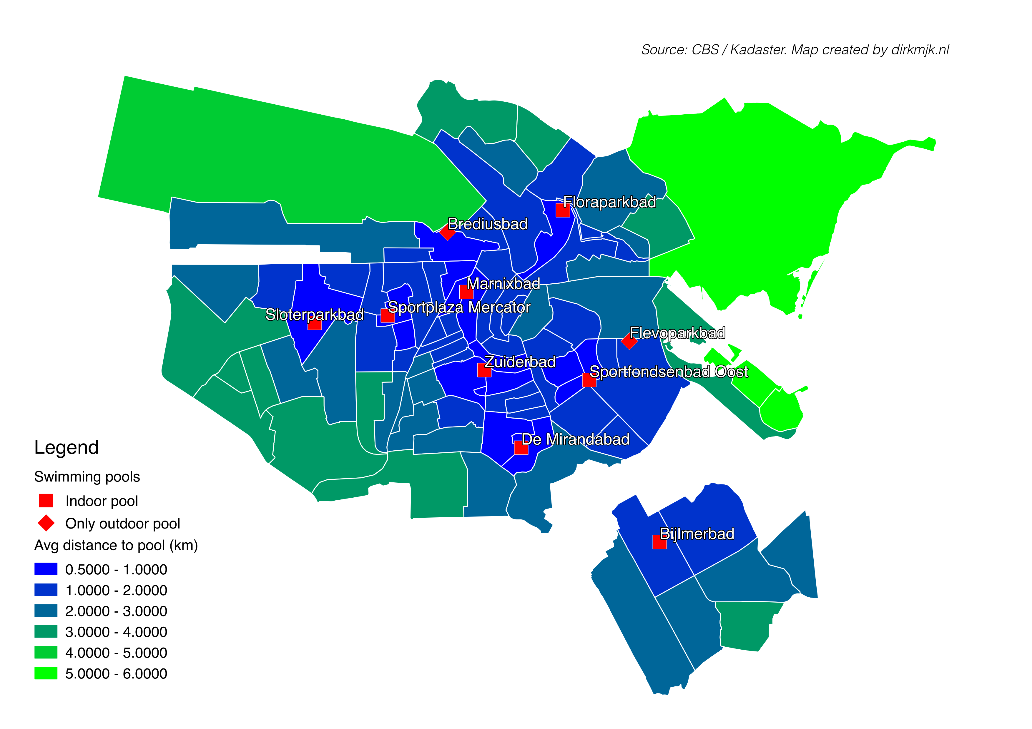
Above is a map of Amsterdam showing the average distance people have to travel to a swimming pool. The map was created with the open source Qgis application and data from Statistics Netherlands (CBS). CBS has data at the neighbourhood level that can be used with a shapefile map they also provide. I’m not very experienced with Qgis and it took me a while to figure out how to create a map with this material. Below I describe the steps that got me there (I use Qgis 2.0.1 for Mac; perhaps things work slightly different in Windows).

CBS data and map

CBS offers data at municipality (gemeente), district (wijk) and neighbourhood (buurt) level on topics including demographics, housing, employment, companies by sector, car ownership, distance to services etc. An Excel file can be downloaded here (select the appropriate year). The same page offers a manual (pdf) specifying which variables are available for which years. To get a general idea of the available data, you could copy the text from the manual and run it through google translate. For technical information, the CBS can be contacted here.

CBS and the Kadaster also offer a map which can be downloaded here. Open the shapefile with the title starting with buurt for the neighbourhood map; wijk for the district map and gemeente for the muncipality map. For the example: below, I’ll use buurt_2011_v2.shp (i.e., the shapefile for version 2 of the 2011 neighbourhood map).

Select a part of the map

The map contains all of the Netherlands, but in this case I’m only interested in Amsterdam. In order to remove the rest of the country:

1. Right click the map layer in the Layers window to the left; select Open attribute table.
2. In the new window that opens, click Toggle editing mode (top left).
3. Click the column name GM_NAME to sort the records by municipality.
4. Scroll down until you reach records for Amsterdam. Select all rows for Amsterdam by clicking them to the left (to do this more efficiently: select the top Amsterdam row; hold SHFT and click the bottom Amsterdam row).
5. Click the button Invert selection; now all but Amsterdam is selected.
6. Click the button Delete selected features. Click OK (it may take a while before all the non-Amsterdam neighbourhoods are deleted).
7. Again click Toggle editing mode; confirm that you want to save the changes to the layer (don’t be shocked if NULL shows up in all cells). Close the window. Right click the map layer in the Layers window and select Zoom to layer extent. You now have a map of Amsterdam.

.

Join with other CBS data

The Neighbourhood and District Map of the CBS contains many data as is. The 2011 version I’m using contains the distance to nearest swimming pool, so there’s strictly no need to join the map with other data. I’ll nevertheless describe the steps to do so, in case you find yourself in a situation in which you do need to add more data to the map. If you whish, feel free to skip this section.

1. Use the CBS Excel file refered to above. The variable we’ll use is AF_ZWEMB (average distance to the nearest swimming pool in kilometers). The Excel file is rather large; in order to make it manageable you may want to delete irrelevant columns. Next, filter the column GM_NAAM (municipality) by Amsterdam. Then filter the column RECS by Buurt (neighbourhood). Now you only have the Amsterdam neighbourhoods.
2. The column AF_ZWEMB contains two missing values represented by ‘x’. Qgis won’t handle them properly; replace them with a number (e.g. -99999). Don’t forget to change them back later.
3. Oddly, the Excel file doesn’t contain a ready variable that can be used as a key to join the data with the map later. Create a new variable consisting of the letters ‘BU’ plus the values of GM_CODE, WK_CODE and BU_CODE (for example BU03630000 for the neighbourhood Burgwallen-Oude Zijde). You can use Excel’s CONCATENATE function for this. Name the new variable BU_CODE2.
4. Make sure there’s at least one variable to the right of AF_ZWEMB (or add one). This needn’t contain values but must be named.
5. Copy all visible cells to a text editor (perhaps needless to say: not MS Word). Save it as cbs.csv.
6. Check if the file doesn’t use comma’s as decimal marks. If it does, a simple way to fix this is by using search/replace. This will also change comma’s in neighbourhood names into points, but for the current project that’s not really a problem.
7. In Qgis, in the menu bar select Layer -> Add Vector Layer. Click Browse to select a file and indicate you’re looking for Files of type: Comma separated value. Select the cbs.csv file and click OK. A new layer has been added to the Layers window.
8. Double click the map layer added earlier. Click Joins to the left of the new window. Click the plus-sign to the bottom of the window. A new window named Add vector join will open. At Join layer, the cbs.csv file is probably selected; that’s ok. The Join field and Target field options should contain identical variables to be used as key variable for the join. Select BU_CODE2 for Join field and BU_CODE for Target field. The click OK twice.
9. In the Layers window, right click the map layer and select Open attribute table. Check if the variables from the cbs.csv file have been added to the right of the table. Among others, you should find the variable cbs_AF_ZWEMB there, as well as at least one more variable to the right of it.
10. The cbs_AF_ZWEMB variable is probably left aligned, because Qgis treats joined data as character strings. Click Toggle editing mode. Deselect all rows (button to the top of the window). Click Open field calculator. Type a name for the new variable you’re going to create and specify that it’s going to be a Decimal number with Precision 1. In the box below Expression, fill out the text ‘toreal( "XXX" )’, only replace XXX with the name of the variable to the right of cbs_AF_ZWEMB (I guess this is a bug: in order to select a joined variable it appears you need to enter the name of the variable to the right of it). Click OK.
11. You should now have added a new variable. You might expect this variable to be to the right of the table, but it’s actually between the original variables included in the map and the joined variables. Don’t forget to remove the -99999 values (or whatever you used for the missing values).

Colour neighbourhoods by distance to swimming pool (create choropleth)

In order to colour each neighbourhood by average distance to the nearest swimming pool:

1. Double click the map layer in the Layer window.
2. To the left of the window, select Style.
3. Click Simple fill. Click the black box next to Border and use the colour selector to select white.
4. In the selector, select Graduated; for Column select AF_ZWEMB and for Mode select Pretty Breaks (in other situations, other options may be preferable); select an appropriate color ramp and click Classify. If you’re satisfied, click OK.

Add locations of swimming pools

You’ll need a csv file with at least the coordinates of the swimming pools. If you have the addresses, you can geocode them here (in order to look up more than 5 addresses you’ll need to create a Bing Maps API, see explanation on the website). My file also has the names of the pools and their type (indoor or only outdoor).

1. In the menu bar, select Project -> Project properties. In the new window, tick off Enable ‘on the fly’ CRS transformation. For CRS, select ‘Amersfoort / RD New’ (the CRS used by CBS). Click OK.
2. In the menu bar, select Layer -> Add delimited text layer. Click Browse to select the appropriate csv file and click OK.
3. Select the appropriate delimiters and the appropriate values for the X and Y fields. Click OK.
4. When prompted, select the appropriate CRS. Usually, this will be WGS 84 (filter by EPSG:4326). Click OK. The locations should now be marked on the map.
5. In order to format the markings, double click the swimming pools layer and select Style. I choose to use different symbols for indoor and outdoor pools. Select Categorized. For column, select Type (or whatever name you gave to the variable specifying the type of pool). Click Classify. Double click the symbols in the legend to further format them. If you want to add labels to the markings, click Labels to the left of the window.

Export the map as pdf or image

1. In the menu bar, select Project -> New print composer (or use CMD-P) and give the composer a name.
2. To the top of the new window, click Add new map. Drag the cursor from the top left to the bottom right of the empty box. The map should now appear.
3. If you want a legend, click the button Add new legend and then click where you want it. Other buttons offer more options to add elements to the map.
4. Either click Export as image or Export as PDF.

And you’re done.

About the swimming pools

In case you’re interested in the story behind the map: dozens of Dutch swimming pools may have to close because of the crisis and higher taxes, although it’s expected few municipalities will risk closing a pool before the city council election on 19 March. In Amsterdam, the Oost District Council will decide on swimming pools in early January. It’s expected that closing the Flevoparkbad will no longer be considered, but it’s uncertain whether a new pool will open at IJburg, as projected earlier. The map shows that residents of Waterland and IJburg (to the East and North-East of Amsterdam) have the highest average distance to the nearest swimming pool.